Common preprocessing steps

Reading raw data and plotting

Load the spant package:

library(spant)

Load some example data for preprocessing:

fname <- system.file("extdata", "philips_spar_sdat_WS.SDAT", package = "spant")
mrs_data <- read_mrs(fname, format = "spar_sdat")

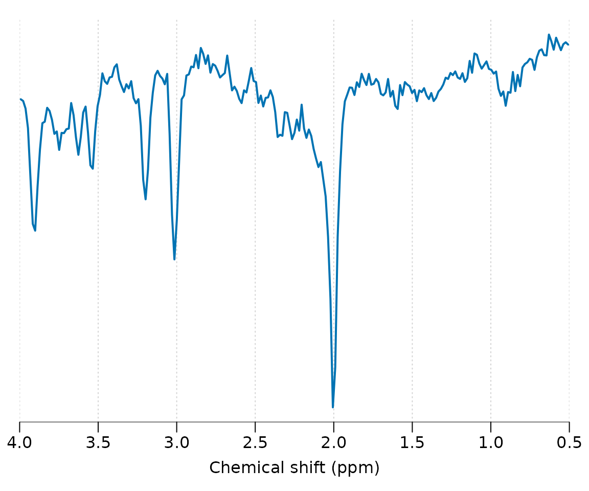
Plot the spectral region between 4 and 0.5 ppm:

plot(mrs_data, xlim = c(4, 0.5))

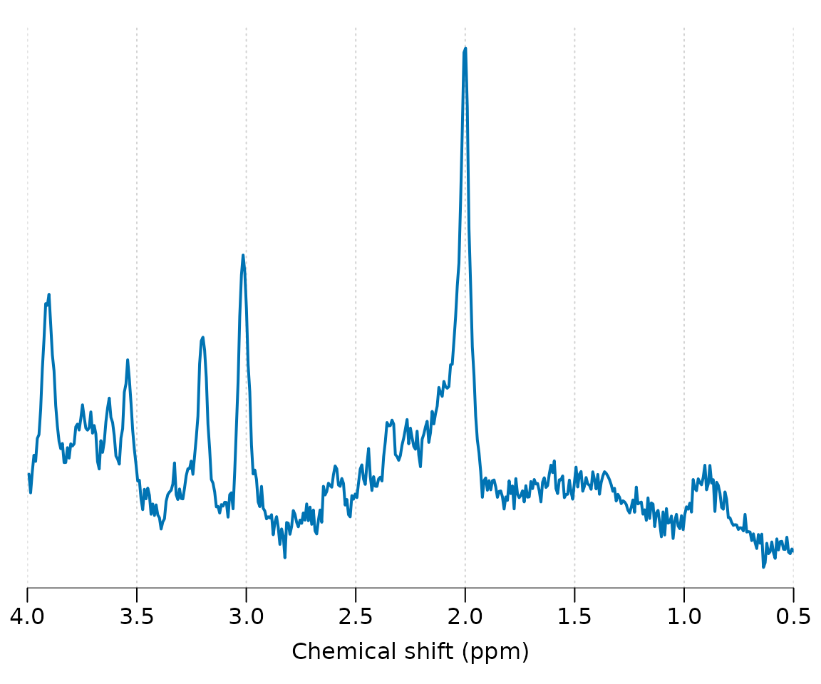
Apply a 180 degree phase adjustment and plot:

mrs_data_p180 <- phase(mrs_data, 180)
plot(mrs_data_p180, xlim = c(4, 0.5))

Apply 3 Hz Guassian line broadening:

mrs_data_lb <- lb(mrs_data, 3)
plot(mrs_data_lb, xlim = c(4, 0.5))

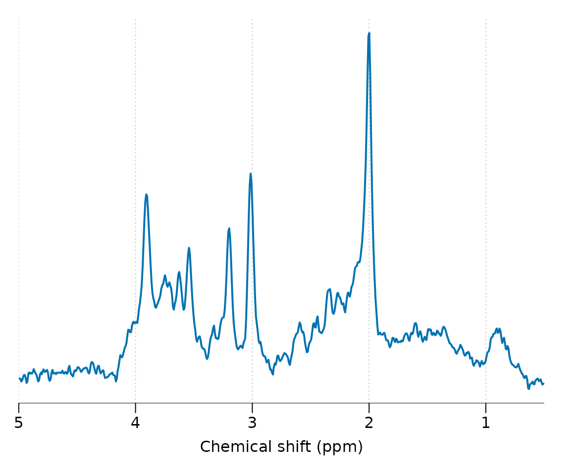
Zero fill the data to twice the original length and plot:

mrs_data_zf <- zf(mrs_data, 2)
plot(mrs_data_zf, xlim = c(4, 0.5))

Apply a HSVD filter to the residual water region and plot together with the original data:

mrs_data_filt <- hsvd_filt(mrs_data)
stackplot(list(mrs_data, mrs_data_filt), xlim = c(5, 0.5), y_offset = 10,
          col = c("black", "red"), labels = c("original", "filtered"))

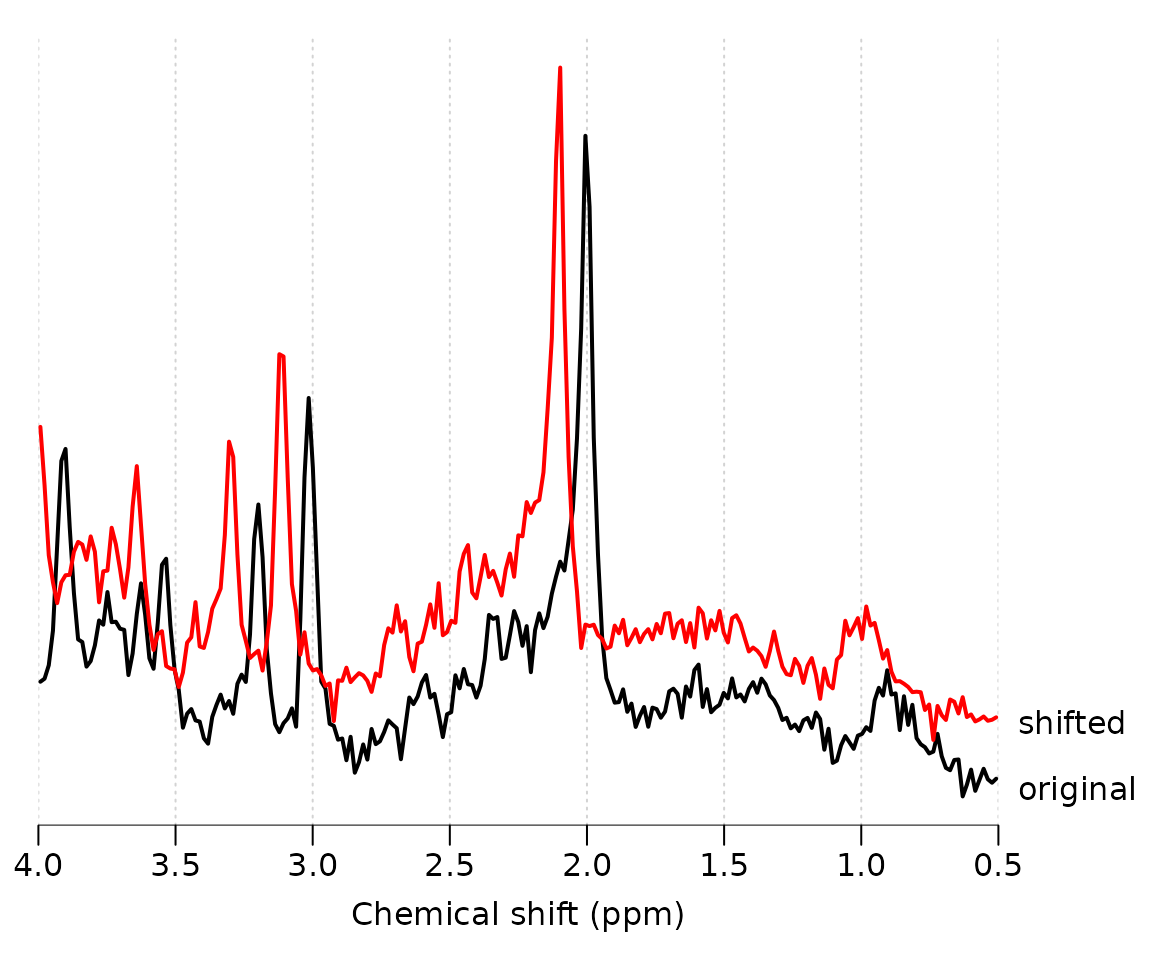
Apply a 0.1 ppm frequency shift and plot together with the original data:

mrs_data_shift <- shift(mrs_data, 0.1, "ppm")
stackplot(list(mrs_data, mrs_data_shift), xlim = c(4, 0.5), y_offset = 10,
          col = c("black", "red"), labels = c("original", "shifted"))

Multiple processing commands may be conveniently combined with the pipe operator “%>%” :

mrs_data_proc <- mrs_data %>% hsvd_filt %>% lb(2) %>% zf
plot(mrs_data_proc, xlim = c(5, 0.5))