fitBsplineObjectToScatteredData — fitBsplineObjectToScatteredData • ANTsR

Fit a b-spline object to scattered data. This is basically a wrapper for the ITK filter https://itk.org/Doxygen/html/classitk_1_1BSplineScatteredDataPointSetToImageFilter.html. This filter is flexible in the possible objects that can be approximated. Possibilities include:

fitBsplineObjectToScatteredData(
  scatteredData,
  parametricData,
  parametricDomainOrigin,
  parametricDomainSpacing,
  parametricDomainSize,
  isParametricDimensionClosed = NULL,
  dataWeights = NULL,
  numberOfFittingLevels = 4,
  meshSize = 1,
  splineOrder = 3
)

Arguments

scatteredData	matrix defining the scattered data input to be approximated. Data is organized by row --> data v, column ---> data dimension.
parametricData	matrix defining the parametric location of the scattered data. Data is organized by row --> parametric point, column --> parametric dimension. Note that each row corresponds to the same row in the `scatteredData`.
parametricDomainOrigin	vector defining the parametric origin of the B-spline object.
parametricDomainSpacing	vector defining the parametric spacing of the B-spline object. Defines the sampling rate in the parametric domain.
parametricDomainSize	vector defining the size (length) of the B-spline object. Note that the length of the B-spline object in dimension `d` is defined as `parametricDomainSpacing[d] * (parametricDomainSize[d]-1)`.
isParametricDimensionClosed	vector of bools defining whether or not the corresponding parametric dimension is closed (e.g., closed loop). Default = FALSE.
dataWeights	vector defining the individual weighting of the corresponding scattered data value. Default = NULL meaning all values are weighted the same.
numberOfFittingLevels	integer specifying the number of fitting levels.
meshSize	vector defining the mesh size at the initial fitting level.
splineOrder	spline order of the B-spline object. Default = 3.

Value

Matrix for B-spline curve. Otherwise, returns ANTsR image.

Details

* 1/2/3/4-D curve * 2-D surface in 3-D space (not available/templated) * 2/3/4-D scalar field * 2/3-D displacement field

In order to understand the input parameters, it is important to understand the difference between the parametric and data dimensions. A curve as one parametric dimension but the data dimension can be 1-D, 2-D, 3-D, or 4-D. In contrast, a 3-D displacement field has a parametric and data dimension of 3. The scattered data is what's approximated by the B-spline object and the parametric point is the location of scattered data within the domain of the B-spline object.

Author

NJ Tustison

Examples


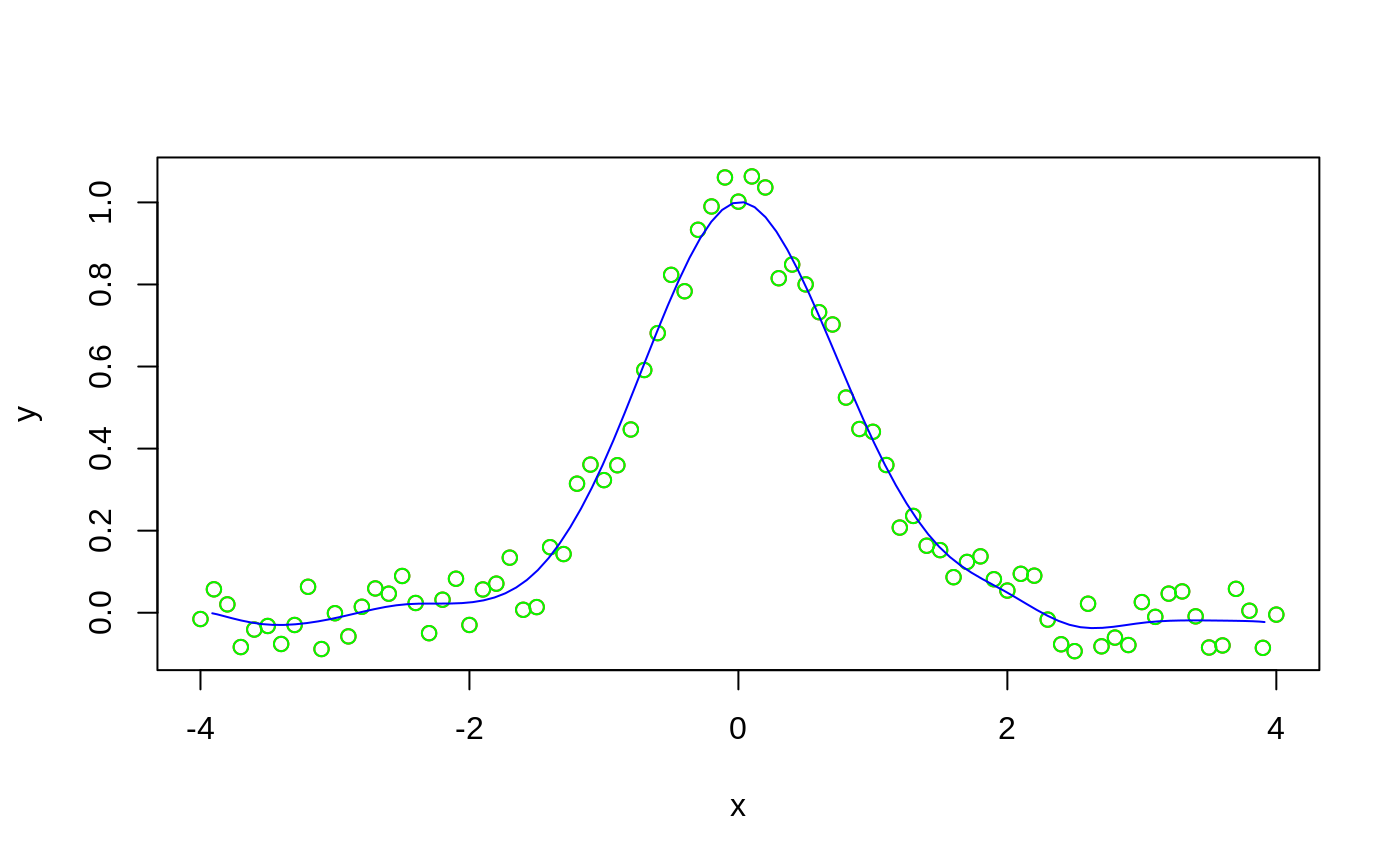
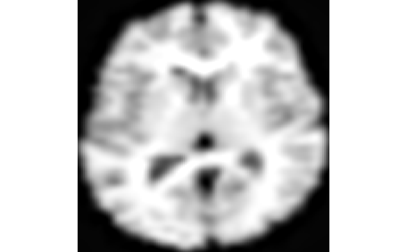
# Perform 2-D curve example

x <- seq( from = -4, to = 4, by = 0.1 )
y <- exp( -(x * x) ) + runif( length( x ), min = -0.1, max = 0.1 )
u <- seq( from = 0.0, to = 1.0, length.out = length( x ) )
scatteredData <- cbind( x, y )
parametricData <- as.matrix( u, ncol = 1 )
numberOfSamplePoints <- 100
spacing <- 1/(numberOfSamplePoints-1) * 1.0;

bsplineCurve <- fitBsplineObjectToScatteredData( scatteredData, parametricData,
  parametricDomainOrigin = c( 0.0 ), parametricDomainSpacing = c( spacing ),
  parametricDomainSize = c( numberOfSamplePoints ), isParametricDimensionClosed = c( FALSE ),
  numberOfFittingLevels = 5, meshSize = 1 )

plot( x, y, "p", col = "red" )
points( scatteredData[,1], scatteredData[,2], col = "green" )
lines( bsplineCurve[,1], bsplineCurve[,2], col = "blue" )

# Perform 2-D scalar field (i.e., image) example

numberOfRandomPoints <- 10000

img <- antsImageRead( getANTsRData( "r16" ) )
imgArray <- as.array( img )
rowIndices <- sample( 2:(dim( imgArray )[1]-1), numberOfRandomPoints, replace = TRUE )
colIndices <- sample( 2:(dim( imgArray )[2]-1), numberOfRandomPoints, replace = TRUE )

scatteredData <- as.matrix( array( data = 0, dim = c( numberOfRandomPoints, 1 ) ) )
parametricData <- as.matrix( array( data = 0, dim = c( numberOfRandomPoints, 2 ) ) )
for( i in seq_len( numberOfRandomPoints ) )
  {
  scatteredData[i,1] <- imgArray[rowIndices[i], colIndices[i]]
  parametricData[i,1] <- rowIndices[i]
  parametricData[i,2] <- colIndices[i]
  }

bsplineImage <- fitBsplineObjectToScatteredData( scatteredData, parametricData,
  parametricDomainOrigin = c( 0.0, 0.0 ), parametricDomainSpacing = c( 1.0, 1.0 ),
  parametricDomainSize = dim( img ), 
  numberOfFittingLevels = 7, meshSize = c( 1, 1 ) )
plot( bsplineImage )
#> NULL