Downloading the data

First, we would like to make sure we have some data to work with. The data is not located directly in the installed package to make it lightweight and some other repository restrictions.

To download the test data, we will use the WhiteStripe function download_img_data:

library(WhiteStripe)
download_img_data()

## [1] TRUE

Getting the filenames

Once the data is downloaded, we can access the files using the ws_img_data function:

files = ws_img_data()

Reading in the data

We will focus on the T1-weighted image here:

library(oro.nifti)

## oro.nifti 0.10.3

t1 = files[grep("T1", basename(files))]
img = readNIfTI(fname = t1, reorient = FALSE)

Displaying the data

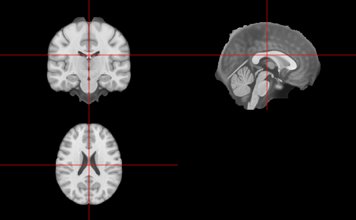
Here we will display the data in 3-dimensions and note that it is a skull-stripped image:

orthographic(img)

vals = img[img > 0]
hist(vals, breaks = 2000)

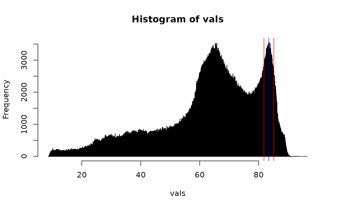
Here we see the distribution of non-zero values. We use 2000 breaks, as this is the default in whitestripe. For T1 images, whitestripe will use the last mode (intensity around 85) in this data.

Running WhiteStripe

Since the image is skull stripped, we will set stripped = TRUE in the whitestripe function:

ws = whitestripe(img = img, type = "T1", stripped = TRUE)

## Making Image VOI

## Making T1 Histogram

## Getting T1 Modes

## Smoothing Histogram

## Smoothing Derivative

## Quantile T1 VOI

names(ws)

##  [1] "whitestripe.ind"     "img.mode"            "mask.img"           
##  [4] "mu.whitestripe"      "sig.whitestripe"     "img.mode.q"         
##  [7] "whitestripe"         "whitestripe.width"   "whitestripe.width.l"
## [10] "whitestripe.width.u" "err"

We see the progress points and the names of the output. This returns the indices of the whitestripe and a mask.img element, which is used to normalize the image:

norm = whitestripe_norm(img = img, indices = ws$whitestripe.ind)

Displaying the output

Location of the white stripe

We can visualize the mode selected and the white stripe:

hist(vals, breaks = 2000)
abline(v = ws$mu.whitestripe, col = "blue")
abline(v = ws$whitestripe, col = "red")

Here we see the blue line for the mode and the red lines for the voxel intensities within the white stripe.

White stripe mask

We can also overlay the mask used for the white stripe:

mask = ws$mask.img
mask[mask == 0] = NA
orthographic(x = img, y = mask, col.y = "red")

We see white matter selected, but the fact that more values within the posterior compared to the anterior part of the brain may indicate a inhomogeneity correction needs to be applied before running whitestripe.

Normalized intensities

norm_vals = norm[img > 0]
hist(norm_vals, breaks = 2000)

Conclusion

Here is a brief overview of the functionality of the WhiteStripe package. Additional information requests are welcome to the bug report/issue page.

Running WhiteStripe on T1- and T2-weighted Imaging

John Muschelli

2021-05-16