Estimate Intrinsic Tissue Relaxivity

Estimation of the intrinsic tissue relaxivity is achieved through nonlinear optimization and the dynamic signal intensities are converted into contrast agent concentration.

R10.lm(signal, alpha, TR, guess, control = minpack.lm::nls.lm.control())

E10.lm(signal, alpha, guess, control = minpack.lm::nls.lm.control())

R1.fast(flip, ...)

# S4 method for array
R1.fast(
  flip,
  flip.mask,
  fangles,
  TR,
  control = minpack.lm::nls.lm.control(),
  multicore = FALSE,
  verbose = FALSE
)

CA.fast(dynamic, ...)

# S4 method for array
CA.fast(
  dynamic,
  dyn.mask,
  dangle,
  flip,
  fangles,
  TR,
  r1 = 4,
  control = minpack.lm::nls.lm.control(maxiter = 200),
  multicore = FALSE,
  verbose = FALSE
)

CA.fast2(dynamic, ...)

# S4 method for array
CA.fast2(dynamic, dyn.mask, dangle, flip, fangles, TR, r1 = 4, verbose = FALSE)

Arguments

signal	is the vector of signal intensities as a function of flip angles.
alpha	is the vector of flip angles (in degrees).
TR	is the relaxation time (in seconds) used in the acquisition of the MRI data.
guess	is the vector of initial values for the parameters of interest: $m_0$ and $R_{10}$.
control	An optional list of control settings for `nls.lm`. See `nls.lm.control` for the names of the settable control values and their effect.
flip	a multidimensional array of contrast agent concentrations. The last dimension is assumed to be a function of the flip angles, while the previous dimenions are assued to be spatial.
...	Additional variables defined by the method.
flip.mask, dyn.mask	is a (logical) multidimensional array that identifies the voxels to be analyzed.
fangles	is the vector of flip angles (in degrees).
multicore	is a logical variable (default = `FALSE`) that allows parallel processing via parallel.
verbose	is a logical variable (default = `FALSE`) that allows text-based feedback during execution of the function.
dynamic	a multidimensional array of contrast agent concentrations. The last dimension is assumed to be temporal, while the previous dimenions are assued to be spatial.
dangle	is the flip angle used to acquire the dynamic MRI data.
r1	is the spin-lattice relaxivity constant (default = 4.39 for 1.5T). For 3T data it may be necessary to adjust this value.

Value

A list structure is produced with (all or some of the) parameter estimates

Scaling factor between signal intensity and T1.

R10

Pre-injection tissue relaxation rate (3D array); $R1_{0}=1/T1_{0}$.

R1t

Time-varying tissue relaxation rate (4D array); $R1(t)=1/T1(t)$.

conc

Contrast agent concentration (4D array).

and information about the convergence of the nonlinear optimization routine.

Details

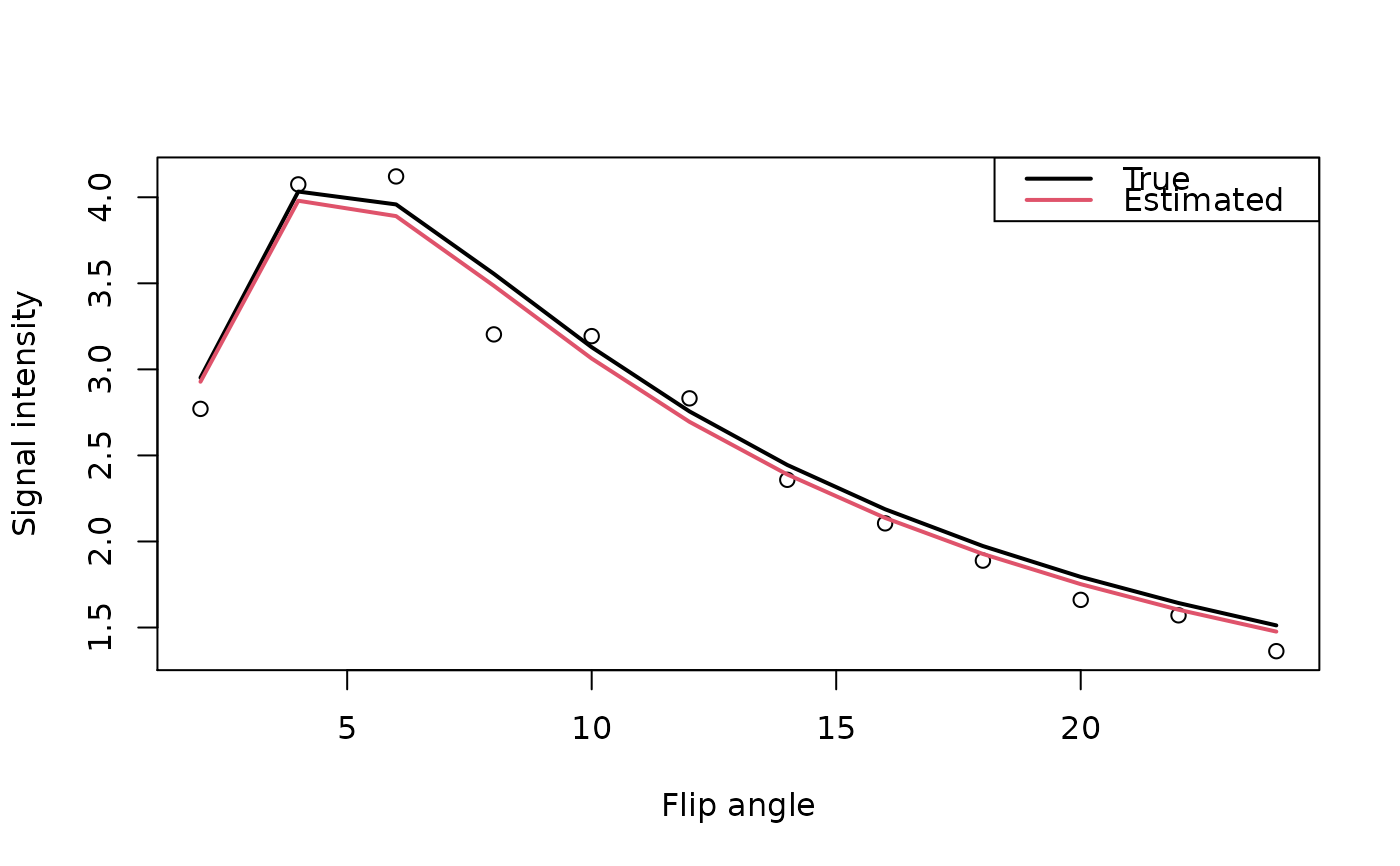
The E10.lm and R10.lm functions estimate parameters for a vector of observed MR signal intensities, as a function of flip angle, using the following relationship $$S(\alpha) = m_0 \frac{\sin(\alpha) \left(1 - \exp{-\textrm{TR}/\textrm{T}_1}\right)}{\left(1 - \cos(\alpha) \exp{-\textrm{TR}/\textrm{T}_1}\right)}.$$ The only difference between the two functions is exactly what is being estimated in the nonlinear least squares formulation. They both require the function nls.lm that uses the Levenberg-Marquardt algorithm.

The CA.fast function calls on R1.fast to rearrange the assumed multidimensional (2D or 3D) structure of the multiple flip-angle data into a single matrix to take advantage of internal R functions instead of loops when calling E10.lm. Conversion of the dynamic signal intensities to contrast agent concentration is performed via $$[Gd] = \frac{1}{r_1}\left(\frac{1}{\textrm{T}_1} - \frac{1}{\textrm{T}_{10}}\right).$$

The CA2.fast function assumes only two flip angles have been acquired and uses an approximation to the nonlinear relationship between signal intensity and flip angle enable to conversion from signal intensity to contrast agent concentration.

Note

The longitudinal relaxivity is set, by default, to $r_1=4(mM\cdot{s})^{-1}$ which is a reasonable value for gadolinium contrast agents at 1.5 Tesla. Double-check the scanning procedure manual to ensure the correct value is used.

References

Buxton, R.B. (2002) Introduction to Functional Magnetic Resonance Imaging: Principles & Techniques, Cambridge University Press: Cambridge, UK.

Li, K.-L., Zhu, X.P., Waterton, J. and Jackson, A. (2000) Improved 3D quantiative mapping of blood volume and endothelial permeability in brain tumors, Journal of Magnetic Resonance Imaging, 12, 347-357.

Li, K.-L., Zhu, X.P., Kamaly-Asl, I.D., Checkley, D.R., Tessier, J.J.L., Waterton, J.C. and Jackson, A. (2000) Quantification of endothelial permeability, leakage space, and blood volume in brain tumors using combined T1 and T2* contrast-enhanced dynamic MR imaging, Journal of Magnetic Resonance Imaging, 11, 575-585.

Parker, G.J.M. and Padhani, A.R. (2003) $T_1$-w DCE-MRI: $T_1$-weighted Dynamic Contrast-enhanced MRI, in Quantiative MRI of the Brain (P. Tofts ed.), Wiley: Chichester, UK, pp. 341-364.

Author

Brandon Whitcher bwhitcher@gmail.com

Examples


## Parameters for simulated data
S0 <- 100
TR <- 5 / 1000            # seconds
T1 <- 1.5                 # seconds
alpha <- seq(2, 24, by=2) # degrees

## Signal intensities for spoiled gradient echo image
gre <- function(S0, TR, T1, alpha) {
  theta <- alpha * pi/180 # radians
  S0 * (1 - exp(-TR/T1)) * sin(theta) / (1 - cos(theta) * exp(-TR/T1))
}
set.seed(1234)
signal <- array(gre(S0, TR, T1, alpha) + rnorm(length(alpha), sd=.15),
                c(rep(1,3), length(alpha)))
out <- R1.fast(signal, array(TRUE, rep(1,3)), alpha, TR)
unlist(out)
#>         M0        R10 
#> 99.5197735  0.6534572 
plot(alpha, signal, xlab="Flip angle", ylab="Signal intensity")
lines(alpha, gre(S0, TR, T1, alpha), lwd=2, col=1)
lines(alpha, gre(c(out$M0), TR, 1/c(out$R10), alpha), lwd=2, col=2)
legend("topright", c("True","Estimated"), lwd=2, col=1:2)