Bayesian P-Splines for Dynamic Contrast-Enhanced MRI Data

Quantitative analysis of DCE-MRI typically involves the convolution of an arterial input function (AIF) with a nonlinear pharmacokinetic model of the contrast agent concentration. This function takes a semi-parametric penalized spline smoothing approach, with which the AIF is convolved with a set of B-splines to produce a design matrix using locally adaptive smoothing parameters based on Bayesian penalized spline models (P-splines).

dcemri.spline(conc, ...)

# S4 method for array
dcemri.spline(
  conc,
  time,
  img.mask,
  time.input = time,
  model = "weinmann",
  aif = "tofts.kermode",
  user = NULL,
  aif.observed = NULL,
  nriters = 500,
  thin = 5,
  burnin = 100,
  ab.hyper = c(1e-05, 1e-05),
  ab.tauepsilon = c(1, 1/1000),
  k = 4,
  p = 25,
  rw = 2,
  knots = NULL,
  nlr = FALSE,
  t0.compute = FALSE,
  samples = FALSE,
  multicore = FALSE,
  verbose = FALSE,
  response = FALSE,
  fitted = FALSE,
  ...
)

Arguments

conc	Matrix or array of concentration time series (last dimension must be time).
...	Additional variables defined by the method.
time	Time in minutes.
img.mask	Mask matrix or array. Voxels with mask = 0 will be excluded.
time.input	Time in minutes for observed arterial input function (default = ‘time’).
model	Only if nlr = TRUE Response model fitted to the estimated response function. Acceptable values include: "AATH" or "weinmann" (default).
aif	is a character string that identifies the parameters of the arterial input function. Acceptable values are: tofts.kermode, fritz.hansen or observed. If observed you must provide the observed concentrations in aif.observed.
user	...
aif.observed	is the user-defined vector of arterial concentrations observed at time.input (only for ‘aif’=observed).
nriters	Total number of iterations.
thin	Thining factor.
burnin	Number of iterations for burn-in.
ab.hyper	Hyper priors for adaptive smoothness parameter
ab.tauepsilon	Hyper-prior parameters for observation error Gamma prior.
k	Order of B-Splines.
p	Number of knots of B-Spline basis.
rw	Order of random walk prior. Acceptable values are 1 and 2.
knots	Vector of knots. Use this if you need unequally spaced knots.
nlr	If TRUE, a response model is fitted to the estimated response function.
t0.compute	If TRUE, the onset time will be estimated from response function.
samples	If TRUE output includes samples drawn from the posterior distribution for all parameters.
multicore	(logical) use the parallel package.
verbose	(logical) allows text-based feedback during execution of the function (default = FALSE).
response	If TRUE, the response functions per voxel are returned.
fitted	If TRUE, then fitted time curved per voxel are returned.

Value

The maximum of the response function Fp for the masked region is provided by default. Where appropriate, response functions, fitted functions, and parameter estimates (along with their standard errors) are provided. All multi-dimensional arrays are provided in nifti format.

Details

See Schmid et al. (2009) for more details.

References

Schmid, V., Whitcher, B., Padhani, A.R. and G.-Z. Yang (2009) A semi-parametric technique for the quantitative analysis of dynamic contrast-enhanced MR images based on Bayesian P-splines, IEEE Transactions on Medical Imaging, 28 (6), 789-798.

See also

dcemri.bayes, dcemri.lm, dcemri.map

Author

Volker Schmid volkerschmid@users.sourceforge.net

Examples

data("buckley")
xi <- seq(5, 300, by=5)
img <- array(t(breast$data)[,xi], c(13,1,1,60))
mask <- array(TRUE, dim(img)[1:3])
time <- buckley$time.min[xi]

## Generate AIF params using the orton.exp function from Buckley's AIF
aif <- buckley$input[xi]

fit.spline <- dcemri.spline(img, time, mask, aif="fritz.hansen",
                            nriters=125, thin=3, burnin=25, nlr=TRUE)
fit.spline.aif <- dcemri.spline(img, time, mask, aif="observed",
                                aif.observed=aif, nriters=125, thin=3,
                                burnin=25, nlr=TRUE)

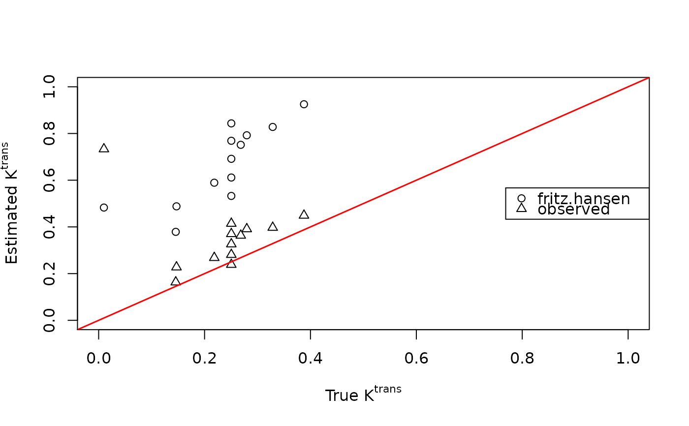
plot(breast$ktrans, fit.spline$ktrans, xlim=c(0,1), ylim=c(0,1),
     xlab=expression(paste("True ", K^{trans})),
     ylab=expression(paste("Estimated ", K^{trans})))
points(breast$ktrans, fit.spline.aif$ktrans, pch=2)
abline(0, 1, lwd=1.5, col="red")
legend("right", c("fritz.hansen", "observed"), pch=1:2)